A Bayesian Calibration Framework for EDGES
The stage is set
In 2018, the EDGES collaboration shook up the field of 21cm cosmology with the first reported evidence that they may have detected the signature of the birth of the first stars. It was big news (at least in our niche little community), not least because the detected “signature” was just the right mix of both conforming to expectation and completely defying it.
For those unacquainted with 21cm cosmology, the EDGES radio telescope is one of a handful of low-frequency single-element telescopes dedicated to observing the the average “brightness temperature” of neutral hydrogen arising from “Cosmic Dawn” (the period in the Universe’s history when the very first stars fired up). The key point here is that these radio telescopes don’t intend on seeing these early stars directly. Instead, they intend on observing what the new kinds of radiation from these stars do to the surrounding gas. This surrounding gas is predominantly neutral hydrogen (that is, the atom with a single proton and a single bound electron). Usefully, neutral hydrogen (or ‘HI’ as we usually refer to it) every now and then spontaneously emits light at a single frequency: 1420 MHz, corresponding to a wavelength of 21 cm.
While this spontaneous emission happens very infrequently, there’s enough HI sitting around that we expect a decent amount of total emission. Exactly how much emission of course depends on all the thermal processes going on in and around the gas – are X-rays from early black holes heating it up? Is the kinetic temperature of the gas low or high? By measuring how much emission there is, we can get a handle on these physical processes. In particular, when stars turn on, their Lyman-alpha emission should cause a net decrease in emission of the 21cm radiation from the surrounding gas. When viewed as evolving over cosmic time, we should thus expect to see a “dip” in the 21cm signal (which eventually rises again due to X-ray heating).
Global signal experiments can view this evolution over cosmic time by measuring a wide range of frequencies (eg. EDGES-low measures between 50-100 MHz) all at once. Frequencies map to cosmic time via the redshift effect of cosmic expansion.
What EDGES saw was a significant dip – right about the time when we expect the first stars to appear (about 300 million years after the Big Bang). What was surpising was that the dip was so deep. In fact, it was so deep that we don’t know of any standard physics that could cause it to be so. This led to a series of suggestions of interesting new physics, like dark matter particles that are oh-so-slightly electrically charged.
The problem is that doing this experiment is really, really, hard. While the dip was much larger than expected, it is still an extremely tiny blip compared to the emission coming from our own Galaxy. Like a tiny imperfection on the otherwise smooth surface of a mirror – only this imperfection is at the level of one part in a hundred thousand. Thus, the issue is: what if we inadvertantly (metaphorically) bumped that mirror ourselves when trying to observe the ‘cosmic imperfection’? What if what we’re really seeing is just wiggles from our own telescope?
An improvement on our analaysis
My recent paper has taken a first step in making double-sure that what EDGES is seeing is really from ‘out there’, not ‘down here’. The problem is this: we are pretty sure the Galaxy itself is actually very smooth (in frequency), but we also know that our instrument bumps that smoothness around into shapes that could look more than a little like the cosmic dip. This happens in a lot of ways: the area on the sky that the ‘scope sees changes with frequency, its efficiency also changes with frequency, and we get these pesky signals from Earth itself (you know, your favorite radio station. On top of that, the electronics within the telescope’s signal chain ‘boost’ the incoming signal (for some really good reasons), and we have to figure out exactly what that boost was, so we can undo it. This process is called ‘calibration’.
EDGES is well-known for its exquisite calibration. However, we can never know for certain that we got the calibration right. What if we over-corrected by just 1%? That would obliterate our chances of observing the cosmic dip. How certain do we really need to be that we’re calibrating to a given accuracy? That question is exactly what I tackle in this paper.
In my work, I build a Bayesian model of calibration. In other words, I build a forward-model of what would happen if we were to say the calibration was just a little different than what we said it was. By describing the calibration with a set of parameters, we can “slide” those parameters around, seeing how well the resulting prediction aligns with the data we actually measured. Bayes’ theorem gives a well-formulated rule for telling what level of belief we should maintain in a certain choice of parameters, given how well its prediction aligns with the measurements. The details are somewhat tricky, but the concept is very simple.
So, what were the results?
I did the work in two parts: first, I propagated our uncertainty on the calibration parameters only against data that we take in the lab purely for calibration purposes. This revealed a slight hitch in the plan: under my model, Bayes’ rule was telling us that the best set of parameters were significantly different from those that we used in 2018.
To understand why requires a little bit of understanding about the calibration process. As I said earlier, the electronics boost the incoming signal by some unknown factor (known as the ‘calibration gain’). To determine this ‘gain’, we take the electronics (called the ‘receiver’) back to the lab, and inject signals from known sources into it in place of the actual antenna. We use four different sources that have characteristics designed to help us get the best handle on the calibration gain (which is not a single number, but rather a number for each frequency). We combine these lab-measurements to determine the gain. However, problematically, two of the input sources are way more tricky to measure than the other two. Traditionally, we’ve tried to minimize the impact of these two sources on the solution for the gain – they’re necessary, but only for part of the solution. However, implementing this same impact-reduction under a Bayesian model is much tougher. This is not a defect in the Bayesian model, but rather a feature – in effect, it makes you do the right thing: it says “if you think there might be something wrong with your measurement of those two sources, give me a model for how you think they might be wrong”. If you can provide such a model, the inference from Bayes’ theorem is gauranteed to be correct (that is, you’ll end up having the right level of belief in your final answer). In practice, in this case it was really tricky to come up with a model for how these two sources might be biased. So, we used a trick: we downplayed their impact in exactly the same way that EDGES always has, and brought their expected measurements back into the Bayesian model. All-in-all, this point was one of the most interesting of the whole work for myself, and is something that needs to be followed up in the future.
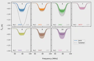
After performing this trick, we propagated the full uncertainty on our calibration parameters through to the data from the antenna itself. Here, we found that the uncertainties on the gains were almost insignificant on our interpretation of the cosmic signal. That is, if we changed the calibration gain within the range it could practically be, given all the data from the lab, the measured “dip” didn’t budge much at all. We found that the (slightly) increased flexibility in the calibration model (compared to the traditional EDGES analysis, which had said that the calibration gain must be exactly that measured in the lab) did help in fitting the sky data when the model for Galaxy emission was not flexible enough. In these cases, the calibration gain model ‘stepped in’ and did some of the work the Galaxy model really should have done. But once the Galaxy model was flexible enough, the calibration gain model settled back down to what we always thought it had been, and nothing really changed.
So, does this confirm the original reported detection? Far from it – this is just a first step. We’ve let the calibration gain model be more flexible, but there are other effects of the instrument (like the changing viewing area per frequency) that we haven’t covered in this new framework yet. And there’s always that pesky situation with those two calibration inputs. Here’s to future work!